Whittle : EXTRAGALACTIC ASTRONOMY


4. LUMINOSITY FUNCTIONS


(1) Introduction
Galaxies come in a huge range of luminosity and mass : ~106 (MB -7.5 to -22.5).
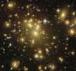
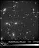 Look at any galaxy cluster, and you see a wide range of galaxy luminosities
[image]
Look at any galaxy cluster, and you see a wide range of galaxy luminosities
[image]
The Luminosity Function specifies the relative number of
galaxies at each luminosity.
The Luminosity function contains information about :
- primordial density fluctuations
- processes that destroy/create galaxies
- processes that change one type of galaxy into another (eg mergers, stripping)
- processes that transform mass into light
Although this information is (badly) convolved, nevertheless :
-
Observed LFs are fundamental observational quantities
-
Successful theories of galaxy formation/evolution must reproduce them

(2) Brief History
1930 Hubble notes that apparent magnitude correlates tightly
with redshift (fainter galaxies have higher z).
He concludes galaxies have a narrow (Gaussian) absolute magnitude
distribution:
<MB> ~ -18,  ~0.9mag
1942 Zwicky realizes that the Local Group contains many low luminosity
galaxies
He argues for a rising function for low luminosities.
As we shall see, this disagreement foreshadows two important facts :
- corrections for sample bias are essential
- there may be two types of LF; one for "normal" galaxies and
one for "dwarfs"
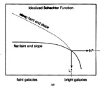
(3) The Schechter Function

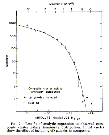 In 1974 Press and Schechter calculated the mass distribution of clumps emerging from the young universe, and in 1976 Paul Schechter applied this function to fit the luminosity distribution of galaxies in Abell clusters [image]. The fit turned out to be excellent, though the reasons why are still not well understood (see sec 7).
 |
(4.1) |
- The function has two parts and three parameters: [image]
- Integration over number gives:
 |
(4.2) |
 where
where  (a) is the
gamma function [image]
and
(a,b) is the
incomplete gamma function.
(a) is the
gamma function [image]
and
(a,b) is the
incomplete gamma function.
For L  0, the total number of galaxies, Ntot = n* (
 + 1).
+ 1).
Note that for
 -1, Ntot
diverges (many many dwarfs)
-1, Ntot
diverges (many many dwarfs)
In reality, the LF must turn over at some lower L to avoid this
- Integration over luminosity gives :
 |
(4.3) |
Integrating from zero gives a total luminosity density of
Ltot = n* L* ( + 2)
For typical , the luminosity does not diverge (nor does the mass)
- Note that the integrated global LF gives a cosmologically important number:
for
= -1, the luminosity
density is ~108 h
LB Mpc-3 , which for M/L ~ 10 gives:
a total mass density of ~ 109 h
M
Mpc-3 , corresponding to
 * ~ 0.004
We conclude that stars/galaxies contain ~10% of all baryons (since bary ~ 0.04)
(The rest is thought to be in the IGM).
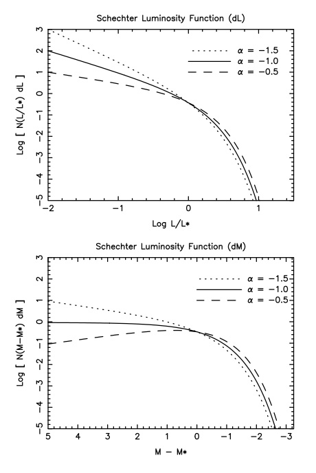
- Be careful which version of the luminosity function is used: [image]
-
 (L) per dL, [which is usually plotted Log () vs Log L].
- (M) per dM where M is Absolute Magnitude, so this is effectively d(logL).
- Sometimes the cumulative LF is given: N > L or N < M.
- Observationally, it is also important to specify:
- whether the LF is for specific Hubble Types, or integrated over all Types
- whether the LF is for Field galaxies or Cluster galaxies (or
whatever the environment is)
- the value of Ho, since
varies as h3 while
L or M vary as h-2 where h = Ho/(100 km/s/Mpc)
(4) Methods of Evaluating Luminosity Functions
Cluster and field samples require quite different approaches:
(a) Cluster Samples
Since all cluster galaxies are at the same distance:
- bin galaxies by apparent magnitude, down to some limit, to get
(m)
- use cluster redshift (distance) to get, simply,
(M)
- Fit a Schechter function to (M)
by minimizing
 2 to obtain M* and
.
2 to obtain M* and
.
Complications arise principally from trying to eliminate fore/back-ground
field galaxy contamination:
- velocities useful (though may still be ambiguous; dwarfs are too faint to
measure)
- dwarfs (except BCDs) have low SB, while distant background
galaxies usually have high SB
- apply statistical corrections to N(m) using field samples.
(b) Field Samples
In general, deriving LFs for the field is more difficult than for clusters:
Many methods have been developed, here is the simplest:
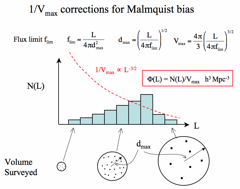
(i) Classical Method (eg Felten 1977)
Obtain a flux limited sample: all galaxies brighter than given magnitude limit.
Use distances to calculate luminosity of each galaxy
Form a histogram in luminosity: N(L).
However, each luminosity bin comes from a different survey volume (Malmquist bias):
[image].

e.g. surveyed volume, Vmax(L), is small (large) for low (high) luminosity objects
So divide N(L) by Vmax(L) to create (L) the density of objects at each luminosity.
This now corrects the Malmquist bias and each luminosity samples the same effective volume.
Unfortunately, this method assumes a constant space density
For nearby samples, this isn't such a good approximation.
(ii) Maximum Likelihood Method
Most modern work uses a "maximum likelihood" approach (e.g. SDSS).
A flux limited sample is a list of galaxies, each with distance di and luminosity Li
Consider the minimum luminosity, Lmin(di), that could be in the sample, i.e. above the flux limit.
The relative number of galaxies of any luminosity that could be at that distance, di is:
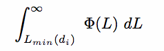 |
(4.4) |
So the probability, pi, that the galaxy actually has luminosity Li is given by:
 |
(4.5) |
One now defines a liklihood function,  , giving the joint probability of finding all Li at their respective distances di:
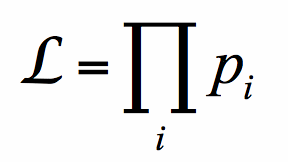 |
(4.6) |
If (L) is parameterized by a Schechter function, then one varies L* and so as to maximize .
These are now the most likely parameters consistent with the data and a Schechter form.
 One can fit any function this way: e.g. a set of values of k(L) specified at K luminosity bins: k (k=1,2,3....K).
This is how the SDSS data were analyzed by Blanton et al 2003: o-link [image]
(iii) Testing Completeness with < V/Vmax >
In addition to Malmquist bias, samples can be incomplete for other reasons:
- magnitude errors near mlim include fainter galaxies
- often, magnitude corrections (e.g. for internal absorption) are only applied
after the sample is defined
In practice, magnitude dependent weighting factors are applied to compensate for the incompleteness.
It is possible to check for completeness with the V/Vmax test:
For each galaxy, find the ratio V / Vmax where:
- V is the volume out to that galaxy
- Vmax is the volume out to dmax, the distance that the galaxy would be at the flux limit.
If the average of that ratio, < V / Vmax > = 0.5 then the sample is complete.
One can also separate the sample into bins of apparent magnitude,
When < V / Vmax >m begins to deviate from 0.5 you've hit the completeness limit of the survey.
Unfortunately, this test also assumes a constant space density.
(5) Different LFs for Different Hubble Types
Early work showed :
- Schechter function is a good fit to many galaxy samples, but
- the parameters (L*,
) can vary depending
on : sample depth, cluster or field, cluster type
Recently, things are becoming clearer :
- it is important to consider the LFs of different galaxy Types.
- it now seems that the LFs of the major galaxy types are
- different from eachother
- relatively independent of environment
- it is the relative proportions of each galaxy type that vary
between cluster and field (see next section)
More specifically, broken down by type, we have the following LFs :
- Spirals (Sa - Sc) : Gaussian, <MB> ~ -16.8 + 5log(h), ~ 1.4 mag
- S0 galaxies : Gaussian, <MB> ~ -17.5 + 5log(h), ~ 1.1 mag
- Ellipticals : Skewed Gaussian (to bright), <MB> ~ -16.9 + 5log(h)
- dwarf Ellipticals (dE+dSph) : Schechter function, M* ~ -16 + 5log(h), ~ -1.3
- dwarf Irregulars (dIrr): Schechter function, M* ~ -15 + 5log(h), ~ -0.3
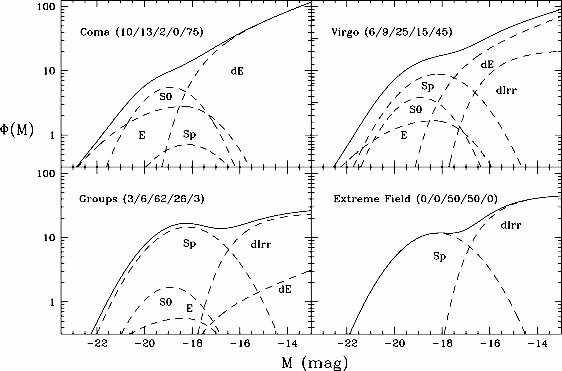
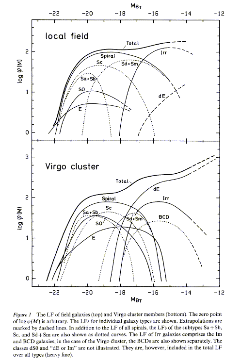 LFs for the Field and Virgo are illustrated here:
[image].
LFs for the Field and Virgo are illustrated here:
[image].
Clearly, full sample LFs :
- have a steep cutoff due to the Gaussian LF of the
luminous Spirals, S0s and Ellipticals
- have rising faint end due to dEs (and to lesser extent dIrr).
(6) Different LFs for Different Environments
It seems the LFs of galaxies in clusters can be different from galaxies in the field.
In general, cluster LFs :
- are well fit by a Schechter function
- have similar L*, though can vary, and is often steeper than in the field (~ -1.3)
- there can be a dip/drop near MB ~ -16 + 5log(h)
- there can be an excess at higher luminosities
- cD galaxies (~10L*) dont fit, and would be considered outliers
in any smooth distribution.
We can now understand much of this :
- different LFs usually arise from different proportions of Sp,
S0, E, dE, and dIrr
- specifically, more E, S0, dEs are in clusters, while more Spirals and
dIrr are in the field,
this is evidence for a morphological dependence on galaxy density [image].
- the dip at MB ~ -16 occurs at the changeover from "normal"
to "dwarf" galaxies
- cD galaxies have clearly had a different history, probably growing by
accretion in dense galactic environments [image]
Analysis of the SDSS shows similar results, but cast in terms of the red and blue sequences [image]
- At higher galaxy density, the relative populations of red and blue galaxies shifts
- There are more high-luminosity red galaxies
- This is consistent with a transformation from blue sequence to red sequence
See
Topic 13 § 7 for a discussion of the physical origin of the morphology-density
relation.
(7) Physical Origin of the Luminosity Function
Why does the galaxy luminosity function have the form that it does?
A complete understanding of this is not yet possible, but here are the ingredients:
Making galaxies involves at least two things
- dark matter halos must form (relatively straightforward)
- baryons must fall in and make stars (complex physics)
Here is a very brief account:
 L
L